The Anatomy of a Variogram
Variograms are a cornerstone of spatial statistics, and are used to describe the variability between data points within a data set as a function of the distance that separates them. Variograms become of critical importance in most geomodelling workflows which use Kriging, as they can describe how much weight to apply to datapoints when predicting values in unknown locations. This post will introduce you to the basic concepts of variogram analysis- What is a variogram, the difference between the experimental variogram and model variogram, and the important parameters of a variogram.
Table of Contents
- What is a variogram?
- Experimental variogram
- Model Variogram
- Sill
- Range
- Nugget
- Discussion
- Further Reading
What is a variogram?
A significant part of geostatistical modeling involves finding quantitative measurements to describe the spatial correlation of a dataset. To understand what this means, consider these two representations of a rock property (in this case, porosity, but it could be anything)
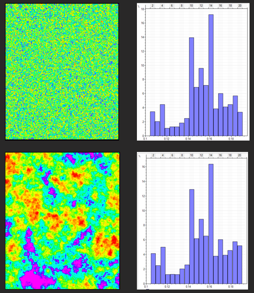
Note first that their histograms are virtually identical; both have the same mean, and variance. However, it’s obvious that there is something fundamentally different. The difference between these two grids is one of spatial correlation. The top image lacks any spatial correlation, and is essentially drawing random values out of a distribution. The bottom image seems to have some underlying pattern, while also containing some degree of randomness as well.
In most situations involving spatial data, measurements made close to each other will generally be more similar than measurements made at a distance. For instance, two wells drilled 20 feet apart will have more similar well log measurements than two wells drilled on opposite sides of a field. The probability of randomly selecting a two star trek fans near a sci-fi convention are far more likely than randomly selecting two star trek fans living 400 miles apart.
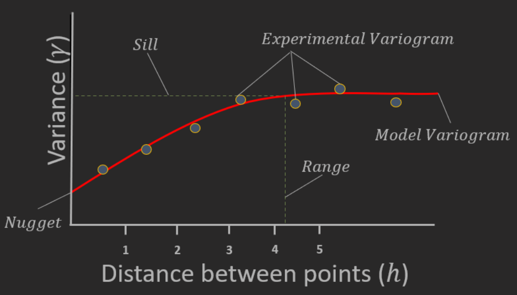
The variogram is the most common method of measuring and modeling spatial correlation and is an essential measurement for running any Kriging based algorithm for estimation or simulation of rock properties. At its core, it’s a graph describing the variance of a dataset with respect to the distance between two data points.
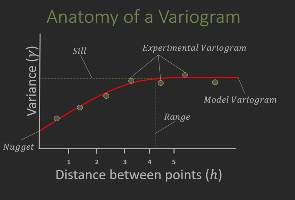
At close separation distances, we see less variance, and thus the items are more similar. As the separation distance increases, we see an increase in variance, until the points flatten out (ideally; real world data can be complicated!).
The variogram itself can be described with relatively few parameters and concepts, but each are important. Let’s take a look!
Experimental variogram
The experimental variogram is a measurement from a spatial dataset, describing the variance with respect to distance. The equation to construct the experimental variogram is as below
$$\gamma\left( h \right)=\frac{\sum_{i=1}^{n}(X_{i}-X_{i+h})^2}{2n}$$
Where γ is the variance, n is the number of points, and h is the separation distance between two datapoints Xi and Xi+h
For anyone familiar with introductory statistics, this equation should look a little familiar. It is very similar to the equation to calculate the variance of a dataset, seen below
$$s^2=\frac{\sum_{}^{}(X-\mu )^2}{N-1}$$
Where s2 is the variance, X is a datapoint, μ is the average of the dataset, and N is the number of samples in the dataset. The main difference is that now, instead of calculating a single number, we’re calculating a function.
The following gif demonstrates graphically what is going on during the calculation of an experimental variogram using a simple 1 dimensional dataset. First, we decide on a separation distance, commonly referred to as lags. In this case, the log data are sampled at every half foot, so we decide lag 1 constitutes all datapoints .5 foot in distance; lag 2 constitutes all datapoints 1 foot in distance, etc. We find every combination of datapoints within a lag, calculate the squared difference between them, sum them up, divide by 2 times the number of two-point combinations, and plot the result on the graph. Rinse, later, and repeat for lags 2, 3, 4, etc.
Extra Credit: What’s with that extra 2 in the variogram equation?
You might be wondering where that extra 2 in the equation came from-
$$\gamma\left( h \right)=\frac{\sum_{i=1}^{n}(X_{i}-X_{i+h})^2}{2n}$$
why do we calculate the variance, then divide by 2? Without getting into the weeds, this factor is required to relate variance to correlation; Technically, we would call it the semivariance; but common convention in geostatistics uses the two terms interchangeably.
Model Variogram
Once the experimental variogram is computed, the geomodeler must fit the experimental variogram to a model. The model variogram is a mathematical function that describes the variance at every conceivable distance, rather than just at the lag distances. These functions are used in the Kriging system of equations for estimation and simulation of properties in 3D space.
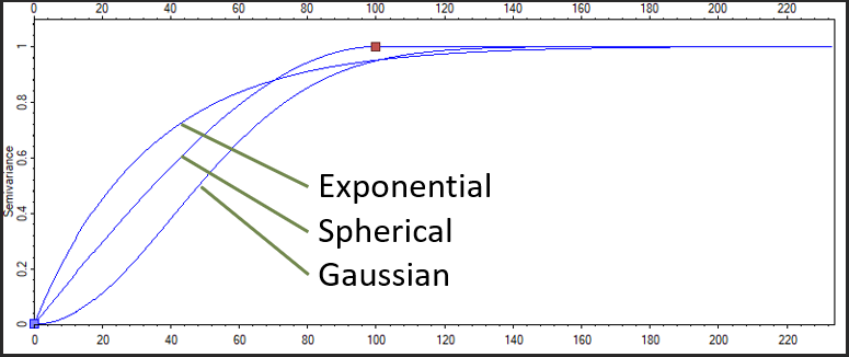
There are many different function types you can use to fit an experimental variogram; the three most common functions being Gaussian, Spherical, and Exponential. , It is also important to note that these functions aren’t geologic in nature- for instance, the spherical variogram model is defined as a function of 1 minus the volume of two intersecting spheres, normalized by the volume of said spheres. It should come as no surprise that the actual equation does not have much to do with, say, the depositional fabric of a prograding deltaic environment. What is important here is to find a variogram model that best fits the experimental variogram (or add up several model variogram functions to create nested variograms! More on this in a future post)
Extra Credit: Model variograms? Why not just fit a line to the points?
The question always arises- If model variograms aren’t geologic in nature, and really don’t have much to even do with variance in general, why do we us them? Why not just fit a line to the points in the experimental variogram, and call it a day? The short answer is that the covariance function derived from the variogram for Kriging must be positive definite, otherwise, weird things happen- and there are only certain families of functions that fulfill this requirement. The long answer requires more math, and will be the topic of a future post.
Once the experimental variogram is abstracted to a model variogram function, it can be described using said function and three additional parameters- the Sill, the Range, and the Nugget.
Sill
The Sill of a variogram is generally considered to be the y-axis value where the experimental variogram points or the model variogram function flattens off at increasing distance; and this should generally happen at the total population variance in a perfectly stationary dataset.
Extra Credit: Sills can act funny in real world datasets
As discussed here, real world datasets are rarely stationary, and sometimes funny things can happen- for instance, you can find datasets that sill out at different values in different directions, or even situations where the experimental variogram never flattens out. These situations will be the topics of future posts.
Many commercial software packages will standardize the variogram function from zero to one, rather than from zero to the population variance. This serves two purposes- one is that when you’re crunching through variogram analysis for multiple rock properties, you don’t have to constantly think about the population variance of each property (simply look for a sill at one!) and two, it directly relates the variogram to the covariance function used in Kriging (more on this in a later post). Just be mindful of this fact!
Range
If the sill is the y-axis value where the variogram flattens out, then the range can be simply considered to be the x- axis value where the variogram flattens out- however that does not convey its true importance. The physical meaning of the range is the distance at which there is no spatial correlation of data. Lag distances greater than the range have no spatial correlation; lag distances less than the range have a spatial correlation related to the variogram function.
Nugget
The nugget is the y-intercept of the variogram, and really describes the variance of a dataset at zero distance. Variance at zero distance? Shouldn’t that always be zero? What does it mean to have variance at zero distance? If I make two measurements of a static dataset at EXACTLY the same location, shouldn’t they be the same? Well, yes and no.
The nugget effect earned its name due to the early history of geostatistics being used in the gold mining industry, and was used to describe the idea that a pure gold nugget could sit a mere centimeter away from regular rock- you have a lot of variance between the properties in very short distances. It seemed like a purely random process with very little spatial correlation. This interpretation of the nugget treats the nugget as a mathematical artifact; It would, in this case, represent the variation of data at distances less than the data sample spacing, simply extrapolated to zero distance.
Another way to interpret the nugget effect, would be the accumulation of tool error. For instance, if you logged a well, then ran the log again, you have measured the same thing, at the same location; however environmental sensitivities, measurement accuracy, etc would almost guarantee subtly different values between log runs. Add to this the fact that throughout the course of the life of an oil field, we use more and more sophisticated (and different) measurement tools, developed by different vendors, different petrophysical studies to calculate rock properties form these logs, and different normalization techniques to quantitatively relate these measurements to a single dataset, you can see how a nugget effect could emerge!
Discussion
The aim of this post is to discuss the basic concepts of a variogram- what it is, and how it’s calculated. The first step in variogram analysis is to calculate an experimental variogram. After this is done, you fit a model variogram to the experimental variogram points, while keeping in mind the sill, the range, and the nugget.
The concepts here generally hold for many datasets, but exceptions in the experimental variogram can be common in non-stationary datasets. For instance, a compaction trend in porosity, where you generally have lower porosity values in deeper rock due to overburden; or a north/south trending turbidite depositing coarse sand in an otherwise shaley environment. These exceptions are not unmanageable, but require some extra considerations, which will be the topic of future posts.
Further Reading
Geostatistics Lessons: Experimental Variogram Tolerance Parameters I only discussed a simple vertical variogram in this post, but in reality you must construct variograms in all three directions. This lesson contains a good discussion on building search cones for horizontal variograms.
Geostatistics Lessons: The Sill of the Variogram This lesson contains more information on how to interpret the sill of a variogram in the presence of trends.
Lazy Modeling Crew: WTF is a variogram? A good introductory conceptual discussion of the variogram, and why it’s important in Kriging.
GISgeography: Semi-Variogram: Nugget, Range, and Sill This post looks at the variogram with GIS and geography workflows in mind, and explains a bit more about common model variogram structures.
