Five Essential Focus Areas in Geomodeling
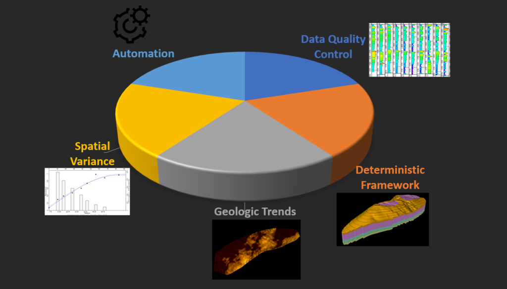
In my last geomodeling post, I talked a little bit about what exactly geomodeling entails. Now I want to step in a bit deeper, and look into what, in my mind, constitute the fundamental focus areas in creating a realistic, functional, and usable 3D geocellular model.
I call these focus areas here rather than phases, because I find that most workflows do not progress cleanly from one area to another- rather, I will often move between them repeatedly, refining and recalibrating different aspects of the model as the project evolves.
In future posts I plan to greatly expand on each of these focus areas; indeed, entire books have been written about each of them- but first, a small taste…
Table of Contents
- Focus area 1: Data Assessment and Quality Control
- Focus area 2: Building the Deterministic Framework
- Focus area 3: Modeling spatial variance
- Focus area 4: Characterizing geologic and spatial trends in the dataset
- Focus area 5: Model Automation/Uncertainty Analysis
- Discussion
- Notes

Focus area 1: Data Assessment and Quality Control
The first focus area is admittedly the least fun, and also admittedly, the area in which you will be spending most of your time and effort throughout a modeling project- sometimes northwards of 80% of your time! This is really due to the sheer amount and complexity of data we collect over a reservoir throughout decades of work. Well logs, seismic surveys, well tops and seismic interpretations, structural maps, core data- the list goes on and on, and the datatypes and variety expand as time marches on and we develop new techniques and measurements.
Part of the job of a geomodeler is to collect and integrate data into a cohesive 3D framework which can incorporate every available geological and geophysical measurement relevant to the study. This means not only doing a full assessment of the amount and variety of data, but calibrating and correcting them as well. In fact truth be told, there are many projects I get involved with which I feel that I never truly escape Data QC Hell.

But do not abandon hope, ye who enter here!
Many data quality problems tend to stand out to a trained eye- For instance, upon importing porosity data, some logs may be referenced to a percent unit with a range of 0-100, and others may reference decimal values with a range of 0-1. Querying your dataset for values outside of a reasonable range, displaying values in a histogram or crossplot, or even creating some preliminary maps from your raw data can make many of these problems stand right out.
Just get comfortable, expect data problems, and stay optimistic- after all, your coffee never gets cold in hell!
Focus area 2: Building the Deterministic Framework
Also commonly referred to as the structural model, the deterministic framework describes the large scale architecture and topology of the region you are modeling. This will include formation boundaries, faults, unconformities, and any notable stratigraphic regions- as well as a grid system bounded by these objects.
The grid system is of critical importance in geocellular modeling, because the size, position, and relationships these cells exhibit will significantly affect the rock property models. By and large, Cartesian grid systems currently dominate the industry- These use hexahedral (six-sided) cell shapes with eight corner points, where cells are arranged out in a 3D array constrained by faults and formation boundaries. When you create rock properties within this grid system, each cell contains a single value per rock property.
There are many things to consider when constructing the framework. For instance, creating a smaller cell size can increase the resolution of the model, but at the expense of computation time (more cells=more math=longer runtime). Another example can be how the cells trend alongside formation boundaries.
Consider the following, where the gold zone and upper portion of the purple zones are truncated by an erosional unconformity. Cell layers can be positioned such that they proportionally follow both the top and base of the zone of interest with a constant number of cells (called proportional layering), or can follow only the base, or only the top of a zone, with a constant cell thickness. The first scenario can be seen on the left hand side, the second to the right.
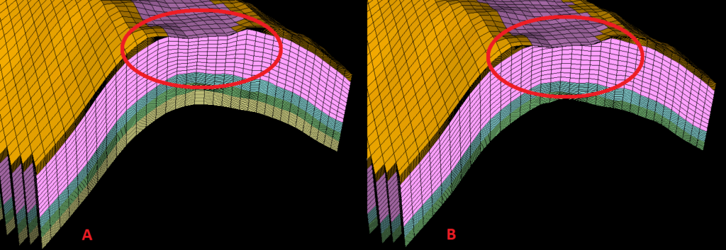
On the left, cells follow the erosional unconformity, and therefore the distributed rock properties will effectively use the erosional unconformity for correlation- log data at the top of the purple zone on the flank of the anticline will be directly compared with well data immediately under the erosional unconformity, deeper into the zone.
On the right, the layers of the model are actually truncated out by the erosional unconformity, and rock properties will follow suit- which is what we want here!
Focus area 3: Modeling spatial variance
This is probably the most abstract focus area when approaching geomodeling from a pure geology or geophysics viewpoint, and that’s because this is where most of your geostatistics come into play. Geostatistics is a branch of statistics which focuses on describing spatial datasets- so instead of looking at a dataset and describing it by a variance, or standard deviation, or even a histogram, we instead look at its variance as a function of distance and direction from known data points, and we use this to make predictions about the distribution of unknown data points throughout the region.
Seem clear as mud? We’ll dig into what precisely this means in a future post when I introduce some geostatistical algorithms and how they are used- but for now, let’s consider the following scenario. We have a dataset that we want to map out across a region (This point set was derived from permeability data, but it really doesn’t matter for our discussion here). Well great- let’s just build a map with minimum curvature, and call it a day:
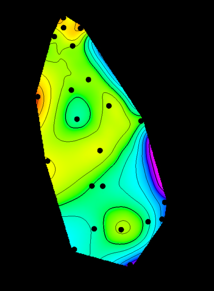
Does this give us anything useful? Well, sort of- we can start to figure out average values across the area, possibly identify spatial trends, etc. But how predictive is this- and moreover, does it really describe the full dataset? Well, for one, rock properties will rarely interpolate linearly and smoothly from one data point to another. The natural geological variation of most rock properties tend to be much, much higher in reality than a simple point to point interpolation can describe. Moreover, when we try to use an overly smoothed map like this in fluid flow simulation, they significantly OVER predict the reservoir’s performance, which would lead to overly optimistic and unrealistic simulation results. In short, while we directly used the data, and we used an industry standard contouring approach for the map, we produced a crappy, unusable result. Something is missing.
Let’s look at this data in another way. This time, we are looking at each data point, and how it relates to each other data point with respect to distance. When we do this, What we would generally expect, is that two points close to each other are more similar than two points further away from each other. In other words, the variance in our dataset increases with respect to distance. Indeed, this is what we see:
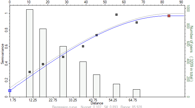
This graph is called a variogram, and it will be the subject of many future discussions as it is one of the most common methods of geostatistical analysis. Variograms are used in every Kriging based algorithm, which is by far still the most common approach used in industry even today. What in essence this tells us though, is how much variance we can expect in different parts of the model, based on the distance to our nearby known datapoints. These are used to weight the known datapoints- plus this approach can be combined with randomness to produce stochastic models- where each time you run, you get a different, but equally probable outcome, like below:
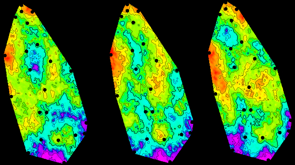
While each outcome looks quite different, what is important here is that we have introduced the variability of the input dataset into the output map- which will give us a much better chance at getting a valid history match out of simulation.
Now this is just one rough example of how geostatistics can be used in reservoir modeling- but you can think of geostatistics for our purposes as a toolbox of methods to produce realistic property models and make statistical predictions, based on your data.
Focus area 4: Characterizing geologic and spatial trends in the dataset
Spatial trends are very closely related to geostatistics, but I split them out as a separate focus area for one important reason- When applied in reservoir modeling workflows, trends are a geologist’s way of imprinting their geologic knowledge onto the model. Allow me to explain.
The vast majority of geostatistical algorithms commonly used in industry make a very important assumption about the dataset being modeled- That is, we must accept the decision of stationary. What does this mean? I will introduce this with more detail in the future, but for now, think of it as meaning that the dataset has a constant mean throughout the region, and a finite variance. In other words, if we dice the model up into smaller regions, we should see *approximately* the same mean within each subregion of the model.
Okay, well what if we have a compaction trend with porosity, where we get porosity reduction due to overburden pressure? What about diagenetic trends? What about depositional characteristics, like for instance we have a sand dominated channel running north-south in our reservoir, flanked by floodplane shales? Or we’re in a shoreface environment, and there are deeper marine sediments flanking one side of the model? There are countless real geologic scenarios which violate the decision of stationarity; Indeed, I very rarely see a real world scenario which CAN be treated as stationary in the geosciences.
So what do we do- take geostatistics and throw it in the dumpster? Of course not- in fact, this apparent problem becomes a strength when used in the right way.
What we do, in fact, is characterize the trend as an expected value, subtract the trend from the dataset, (which sets that dataset as stationary), then add it back after distributing the property. This is simpler than it sounds. In conventional reservoir characterization workflows, we already create maps and functions to describe average changes in rock properties throughout the area of interest (for example, an average porosity map, or net sand map; or a 3D seismic porosity, lithology, or density inversion). These products are by their very nature geostatistical trends, and can be incorporated into a 3D modeling workflow with few modifications. By using them in the model, you actually drive the model with geology, instead of just mathematics.
The general process of trend removal is shown conceptually in the below figure, but note that in most software packages, you need only identify the trend- the removal/restoration process is usually taken care of by the software.
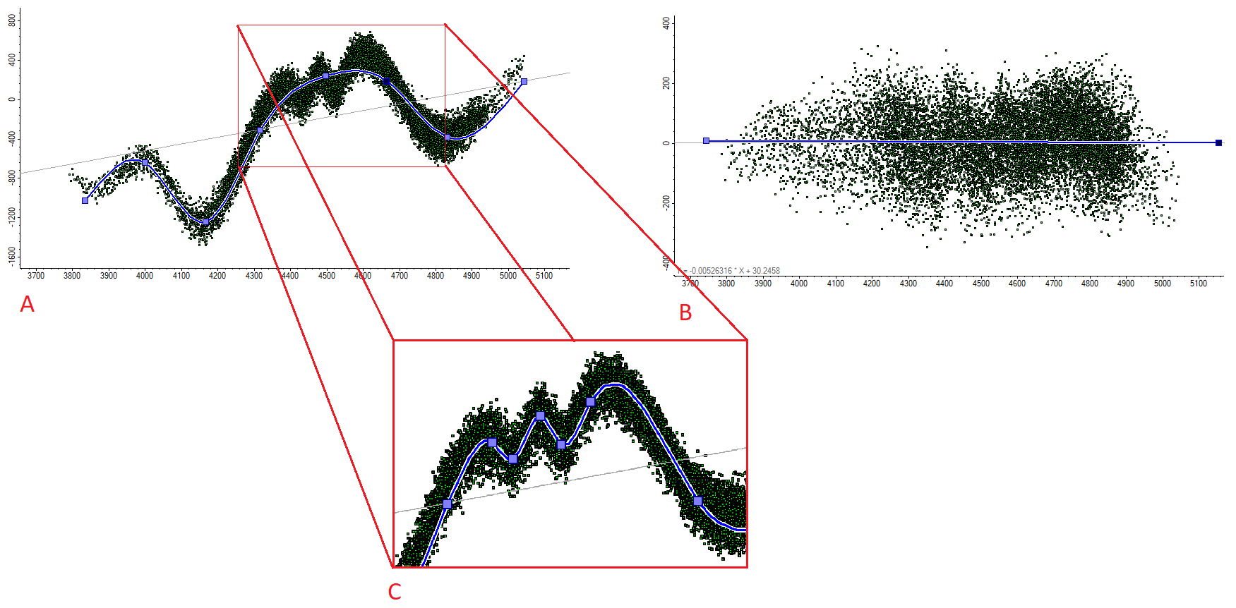
The process of removing a trend from the dataset is done as follows: A) Visualize the data and identify a trend (blue line) – through the data. B) Flatten the trend out to a straight line, and transform the data as well. Once you distribute the property, you run the distributed property back through the transform, restoring the trend. C) Note that the shape of a trend can vary by scale- If we were modeling the entire dataset, we might use the original trend, however if we were building a localized sector model, we might further refine the trend to the one depicted in the thumbnail.
Focus area 5: Model Automation/Uncertainty Analysis
This focus area isn’t as important for short term projects, but becomes absolutely critical when creating Living Earth Models which require regular updates, and for reserve estimation workflows which require uncertainty quantification such as P10/P50/P90 values.
We obtain new data quite frequently. This could come in the form of a newly drilled well, or freshly processed petrophysical logs. Indeed, geologists and geophysicists on your team can update their interpretations on a daily basis, and the model is only as relevant as the data feeding into it. Models which cannot accommodate these data go stale over time, and so you need a way to incorporate these data without spending weeks or months building a new model from scratch.
My philosophy on this matter is to approach model building with a programmatic mindset. Many of the core inputs to 3D modeling require filling out a list of parameters, and hitting execute. Some properties use others as input, and must be updated in a certain order. If you can chain these steps together sequentially, then you can essentially script out the entire model building workflow to run at the press of a button. If you need to fundamentally alter any of the interpretive inputs- for example, a structural map, petrophysical log, or variograms- you can simply add the new input, press a button, and PRESTO- model update complete!
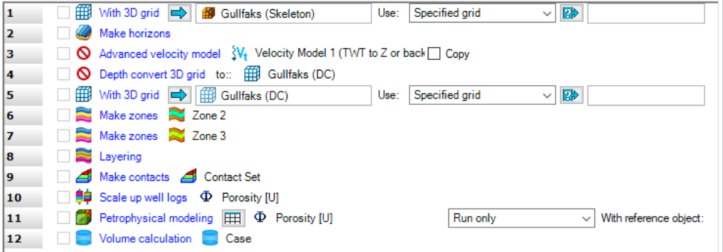
An example of a basic model update workflow. Each step can be modified independently of others, and then the model updated to account for all interpretive and data alterations.
With a programmatically updateable model, you also unlock the possibility of performing uncertainty analysis, by running automated updates hundreds, or thousands of times, with different input parameters each time. Uncertainty analysis allows you to not only determine model accuracy and reliability and assess risk, but allows you to target which exact modeling parameters have the largest effect on your calculation. For instance, with reserve estimation for oil and gas in a conventional reservoir, what effect does uncertainty in your oil/water contact have on oil in place, vs say, the standard deviation of your porosity distribution?
As we dig further into uncertainty in some future posts, you will come to realize that uncertainty analysis is a surprisingly deep and philosophical topic. Quantifying measurement uncertainty, interpretation uncertainty, uncertainties in well logs and petrophysical analysis, and seismic data analysis, can involve a multitude of approaches and inference all its own. However, by building your model with automation in mind, you not only make your life far easier in the long run in terms of weekly to even daily push-button model updates, but open the door to the world of quantifying uncertainty- allowing you to assess the predictive power of your model.
Discussion
As with any brief introduction, I have only barely scratched the surface of each of these five focus areas, and provided a couple rudimentary examples. The deterministic framework will guide and directly affect model property correlation directions and the large scale structure of the model. Assessing the spatial variance and using the toolset of geostatistics allows you to create more realistic rock properties, which also behave properly in dynamic reservoir simulation. Characterizing geological trends within your properties will give you the ability to create geologically driven geomodels, rather than just modeling everything statistically. Model automation and uncertainty analysis extends the life and predictive power of your model. Meanwhile, the specter of data quality control will loom over all aspects of the modeling project at large. With enough knowledge and diligence spent in these five focus areas, you will become a formidable geomodeler!
Notes
Project Data used for images derived from- Teapot Dome, Natrona County, WY
This is a non-proprietary dataset sourced from the U.S. Department of Energy
If you would like more information on identifying and modeling spatial trends, check out this page at geostatisticslessons
Michael Pyrcz, associate professor at UT Austin, also has an excellent free course on data analytics and geostatistics on Youtube. Definitely check that out if you want a deeper dive into this subject.
